MIE444 Maze Rover
MIE444 is a mechatronics course at the University of Toronto where teams build rovers to navigate a maze, locate a wooden block, and deliver it to a drop-off zone. The typical approach was an omni-wheeled bot with ultrasonic sensors, running control logic off-board in a Python script over Bluetooth. Autonomous navigation was originally required, but after milestone 1 many teams were still struggling to get their hardware running, so those marks were moved to bonus.
I came in with a software background and saw this as a chance to push myself. I took on all the control algorithms, firmware, and sensor strategy, and built a fully autonomous system running entirely onboard a Raspberry Pi in Rust.
The maze is 8 by 4 feet. The rover is placed at a starting position randomly selected by the TA with no prior notice, and once placed it is hands off. The loading zone is a fixed 2 by 2 foot area, but the block is placed anywhere within it by the TA. The drop-off location is one of four fixed cells in the maze, selected by the TA and given to the bot just before the run begins.
The video below is from milestone 2, which demonstrated autonomous navigation only. Block pickup was added in milestone 3. This is the milestone 2 hardware revision, which is why the rover looks different from the thumbnail which was milestone 3.
Localization
Localization solves two sub-problems: grid alignment finds the rover’s continuous position and orientation within its current cell, and cell identification determines which cell that is. Together they produce an absolute pose in the maze.
Grid alignment
All LIDAR points in the maze fall on walls, and all walls are built on a 1 foot grid. The rover’s position within its current cell can be read directly from this structure, if you can figure out how the point cloud is oriented relative to the grid.
The key insight is projection. Rather than fitting lines to the 2D point cloud, the algorithm projects all points onto a single axis. When the projection axis is aligned with the grid, walls running perpendicular to it collapse into sharp clusters spaced exactly 1 foot apart. When misaligned, the same points spread into a blur with no clear structure.
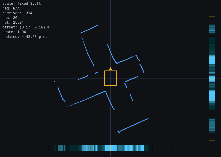
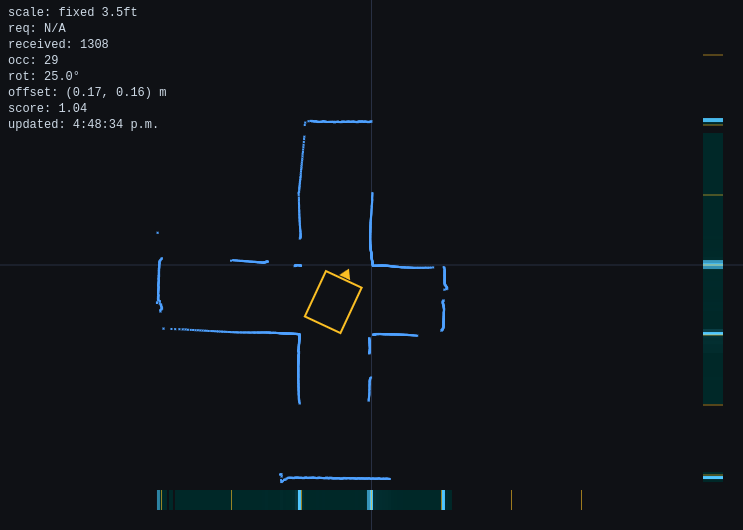
A single-bin Fourier transform at the 1 foot frequency turns this into a measurement. The magnitude tells you how strongly the 1 foot period is present: higher means sharper clusters, which means better alignment. The phase tells you where the first peak sits, which is the sub-cell offset along that axis.
The algorithm tests 180 candidate rotation angles at 0.5 degree increments over a 90 degree range. Only 90 degrees is needed because the maze has two perpendicular families of walls, so the projection pattern repeats every quarter turn. At each angle, the points are rotated, projected, and the Fourier coefficient is evaluated. The rotation that maximizes the magnitude across both axes is the rover’s orientation, and the phase at that rotation gives the x and y offsets directly.
This runs in O(N) time per rotation candidate with no feature extraction or line fitting. Points that do not align with the 1 foot period contribute weakly to the magnitude, so noise is filtered naturally. Processing a full scan of 1600 points takes 55ms.
Cell identification
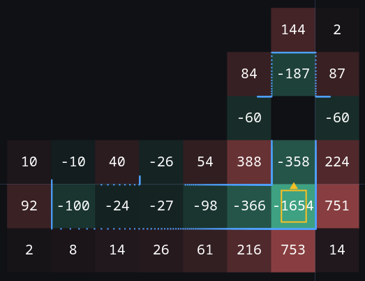
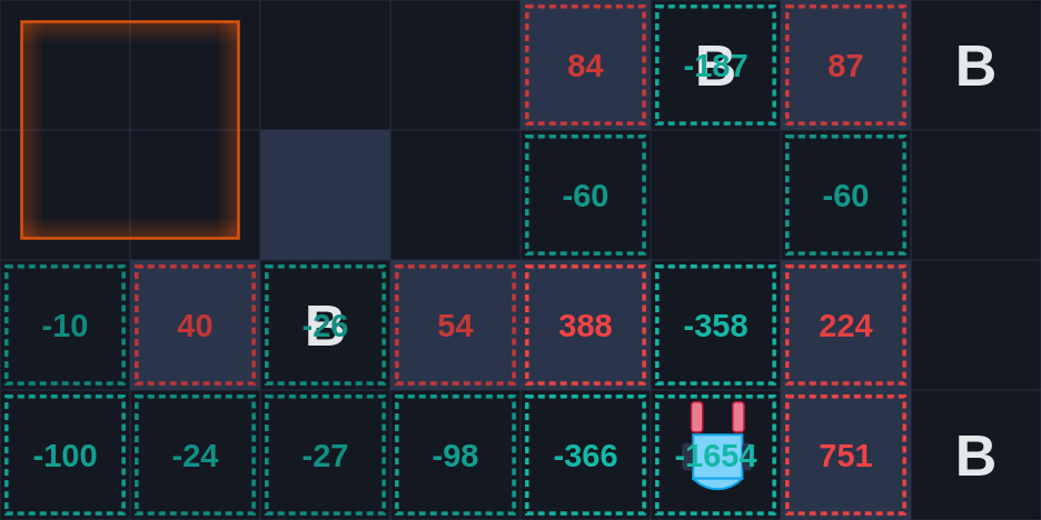
With the point cloud grid-aligned, we build a local occupancy map from each scan. Since all walls are grid-aligned, every LIDAR point must lie on a horizontal or vertical grid line. That grid alignment gives you the wall normal directly: you just determine which axis the point falls on. From the normal you know which side of the wall is filled and which is empty, so each point contributes exactly two observations with no ray traversal needed. This gives a sparse map of the rover’s immediate surroundings with both positive and negative evidence, built in a single pass through the point cloud.
That map is then slid across all 128 possible positions and rotations in the known maze (32 cells × 4 orientations) and scored against the expected maze structure. The highest scoring position is the rover’s current cell. Correct matches typically score between 90% and 98%, and failures are transient, lasting one or two frames before the next scan corrects them. Cell identification takes 1ms.
With around 1600 points per scan and a small maze full of visible walls in every direction, both steps run on a single scan with no accumulation needed. The TA thought we were cheating when he first saw the localization update instantly after the rover was placed, and had us move it to several positions to verify we were not hardcoding a starting point.
Sensor Fusion
The LIDAR runs at 5.5Hz, and scan skew during rotation makes LIDAR-based pose estimates unreliable. A gyroscope running at 200Hz handles heading estimation between scans and during turns. LIDAR corrections are velocity-gated: above an angular velocity threshold, the gyroscope integrates alone. This is safe because navigation always uses in-place pivots, so the rover is never translating while rotating. Gyro drift stayed under 1-2 degrees over 5 minute runs, which was sufficient for reliable navigation.
Navigation
A* pathfinding on the 32-cell grid takes under 1ms and produces a waypoint list through the maze. Collinear waypoints are filtered out, reducing a typical path to 4 or 5 turns.
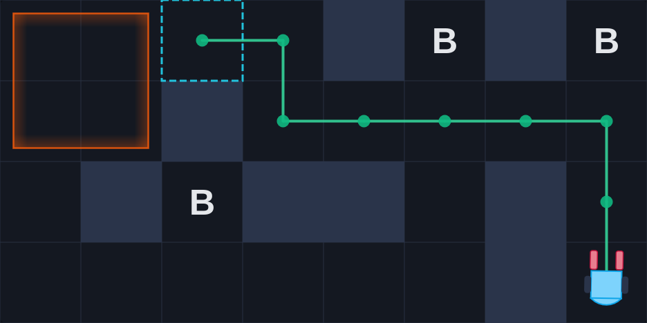
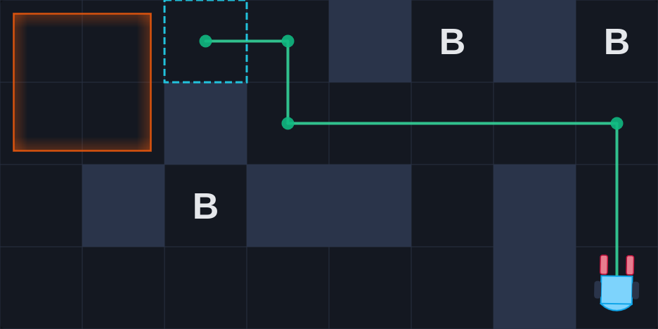
The rover executes the path with proportional control at 50Hz: it pivots in place at each waypoint then drives forward, with forward speed scaled by the cosine of the heading error so it only moves fast when pointing in the right direction.
With absolute positioning from the localization system, proportional control proved sufficient. There is no accumulated drift to correct for, so integral and derivative terms would have added complexity without benefit. Dynamic Window Approach and Pure Pursuit were both evaluated and abandoned quickly in favor of this simpler approach.
Architecture
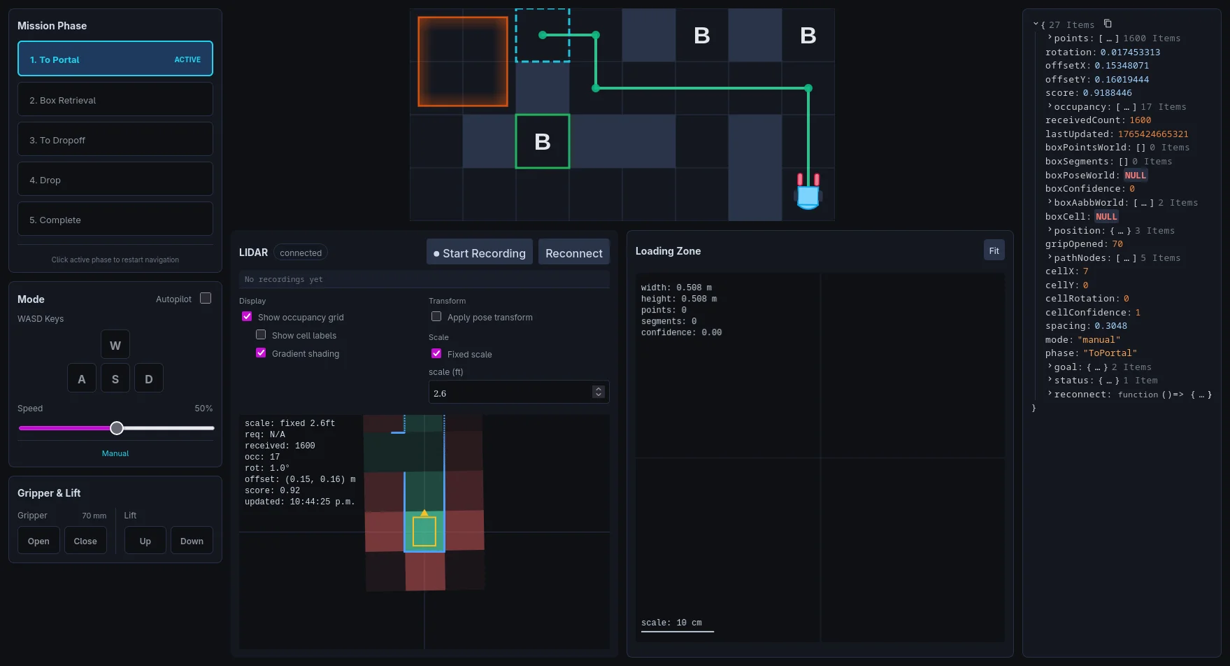
The software is organized into four layers: hardware, control, mission, and interface. Each layer communicates through well-defined interfaces, so changes to one do not ripple through the rest. All hardware components implement Rust traits, allowing a single mode switch to swap between real hardware and a full simulation without touching any algorithm code.
This made rapid iteration possible. The simulation runs the same localization, fusion, and navigation code as the real bot, so algorithms could be validated on a laptop before deploying to hardware. The web frontend was also developed against live simulation data, keeping the full stack exercised throughout development.
Box Detection
Detecting the block required knowing its exact pose to align the gripper. The original plan was three time-of-flight sensors mounted on the front of the rover, but they proved too unreliable to detect the small wooden block consistently.
The alternative was to use the LIDAR for box detection as well. We relocated it from the top of the chassis to underneath, scanning at ground level. Custom large-diameter wheels with thin spokes kept the field of view clear. This is also why the rover in the composite video above looks different from the one in the thumbnail.
For detection, LIDAR points are filtered to the loading zone area in world space. Since the maze contains nothing else at block height, the remaining points belong to the block. A template is then fit to those points to extract the block’s position and orientation.
This worked reliably in initial testing, but the template fitting caused the LIDAR to crash intermittently as the competition approached. Fitting and USB polling ran in a single loop on one thread. As the rover approached the box, more points fell within the loading zone mask, slowing each fit. When the fit ran long enough, the loop fell behind on polling the USB interface, and the LIDAR would crash. The fix was straightforward: downsample the masked points before fitting to keep the loop fast enough to service the USB. I identified this an hour before the milestone 3 demonstration but did not have time to validate the fix, so we ran the mission manually to avoid risking marks on untested code. After the competition I applied the fix and ran the full mission autonomously in the maze I built in my living room.
Results
All three milestones earned full marks. At milestone 1, bonus marks were earned for a second run controlled remotely using only the LIDAR feed, without line of sight to the rover. Milestone 2 is the highlight: the rover localized from a random starting position and completed the course autonomously in 25 seconds with zero collisions, earning bonus marks for autonomous control. Milestone 3 demonstrated full block pickup and delivery under manual control in 2 minutes 18 seconds, driven from across the room without line of sight using only the frontend sensor views. The head TA noted that only one other team in the course’s history had been faster.